How to use VLOOKUP function in excel

How to use VLOOKUP function in excel

Background:

If you are new in excel or you are fresher and have just joined industry, you probably listen words like VLOOKUP on daily basis. Excel is an integral part of our life and VLOOKUP too.  V stands for Vertical. It is vertical look up. By end of Post you will get to know how to use VLOOKUP function in excel.

Normally now a days companies are using SAP or ERP system when they give unique numbers to each item e.g. employee number, material number, customer code, vendor code, GL Code etc.  Such ERP system provide faster report using unique numbers but as an end user we also find ourselves in number games and it is very difficult to recall particular code with its name.

Use of Vlookup:

Let us first understand usage of VLOOKUP function before actually we start working on function. As explained earlier, suppose you want to download stock from your Accounting/ERP SAP System, it will provide list of 1000 items with material code, qty and value but you also requires material name along with material code. You should download master list of material code with material name from your legacy system or you can take help of master data team to download these details.  Generally standard SAP report or some customise report (Y/Z) in SAP don’t carry corresponding name for particular item for faster downloading of report. Here you can use VLOOKUP function to get corresponding name.

VLOOKUP Formulae:

VLOOKUP (lookup_value, table_array, col_index_num, [range_lookup])

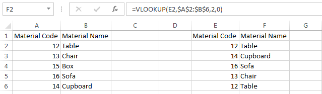
Let us make this formulae very simple. We are asking excel to get name of material against respective material code from master list. See given below screen where simple formulae for VLOOKUP is =VLOOKUP (E2,A2:B6,2,0) to get material name (Table) against material code (12)

Click here to download Excel file to understand and pratice below mention example.

Pre-requisite for VLOOKUP:

Now what is pre-requisite for VLOOKUP is to have master list which is mentioned from A1:B6 , to use $ sign in range if we are using VLOOKUP in same excel workbook. We can break formulae in following four parts for better understanding.

1. E2: provide code for which you required material name
2. A2:B6 : Give range of master data list. Here you have to use $ sign in given range i.e. $A$2:$B$6 if you are using formulae in same excel workbook. One can use F4 before A and B respectively to freeze range. One can directly select entire column instead of freezing range i.e. A:B.
3. 2: while selecting range using this function, we can see column number(2C) where required material name exists against respective material code i.e. second column from left side. For understanding ,we have used data having two columns only but in real life you have to work on data having numerous columns hence we should write number from formulae as depicted in below picture .

4. 0: Using ZERO at last indicates that if excel find exact match for 12 then only it will write name and not if you write 12.25 instead of 12. User can use 1 instead of 0 , excel will provide name as Table even if we have mention 12.25 in cell number E2.

Kindly check below picture for complete use of  VLOOKUP Formulae . We have apply formulae in cell F2 and pasted the same in remaining cell F3 to F6 to bring name of respective material.

VLOOKUP in spreadsheet:

You can copy above details in spreadsheet to understand example better.  Click here to download Excel file to understand and pratice below mention example.Please note that if excel unable to get requested material code in master data, it will throw error as “#N/A”

Hope I am able to explain how to use VLOOKUP function in excel in simple way.  Feel free to give your comments in case of any query or feedback.